Table of Contents
Standard Model
This appendix describes the “standard” nonlinear material model implemented in PMD.
Stress tensor invariants
Let’s define the standard invariants $I_1$, $J_2$ a $J_3$ of the stress tensor $\sigma_{ij}$ \begin{align} I_1 &= \sigma_{kk}=\sigma_{11}+\sigma_{22}+\sigma_{33},\\ J_2 &= \frac{1}{2}s_{ij}s_{ij},\\ J_3 &= \frac{1}{3}s_{ij}s_{jk}s_{ki}=\det\left|\begin{array}{lll} s_{11} & s_{12} & s_{13} \\ s_{21} & s_{22} & s_{23} \\ s_{31} & s_{32} & s_{33} \end{array}\right|, \end{align} where $s_{ij}$ is the deviatoric stress tensor $$s_{ij} = \sigma_{ij}-\frac{1}{3}\delta_{ij}I_1$$ and $\delta_{ij}$ is the Kronecker delta.
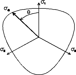
In PMD we use different but equivalent triplet of invariants, namely mean stress $$\sigma_m = \frac{1}{3}I_1,$$ von Mises effective stress $$\sigma_e = \sqrt{3J_2},$$ and Lode parameter $$\mu = \cos(3\theta)=\frac{27}{2}\frac{J_3}{\sigma_e^3}.$$ The angle $\theta$ is directed from the axis of the principal stress $\sigma_1$ to the point representing the stress state in the deviatoric plane, see Fig. 1.
Next, let’s express the derivatives $\sigma_m$, $\sigma_e$, and $\mu$ with respect to $\sigma_{ij}$: \begin{align} \frac{\partial\sigma_m}{\partial\sigma_{ij}} &= \frac{1}{3}\delta_{ij},\\ \frac{\partial\sigma_e}{\partial\sigma_{ij}} &= \frac{3}{2}\frac{s_{ij}}{\sigma_e},\tag{1}\label{1-8}\\ \frac{\partial\mu}{\partial\sigma_{ij}} &= \frac{27}{2}\frac{s_{ik}s_{kj}}{\sigma_e^3}-\frac{9}{2}\frac{\mu}{\sigma_e^2}s_{ij}-3\frac{\delta_{ij}}{\sigma_e}. \end{align}
Consider the special case of uniaxial stress where $\sigma_{11}=\sigma$ and the other components of the stress tensor are zero. Then \begin{align} \sigma_m &= \frac{1}{3}\sigma,\\ \sigma_e &= |\sigma|,\\ \mu &= \pm1. \end{align} The sign $\pm$ of the invariant $\mu$ distinguishes uniaxial tension ($+$) from uniaxial compression ($-$).
For the derivatives in the case of uniaxial stress we have \begin{align} \frac{\partial\sigma_m}{\partial\sigma_{ij}} &= 0 \quad i\ne j,\quad \frac{\partial\sigma_m}{\partial\sigma_{11}} = \frac{\partial\sigma_m}{\partial\sigma_{22}} = \frac{\partial\sigma_m}{\partial\sigma_{33}} = \frac{1}{3},\\ \frac{\partial\sigma_e}{\partial\sigma_{ij}} &= 0 \quad i\ne j,\quad \frac{\partial\sigma_e}{\partial\sigma_{11}} = \pm1, \quad \frac{\partial\sigma_e}{\partial\sigma_{22}} = \frac{\partial\sigma_e}{\partial\sigma_{33}} = \mp\frac{1}{2},\tag{2}\label{1-10}\\ \frac{\partial\mu}{\partial\sigma_{ij}} &= 0. \end{align}
Generalized yield criterion
Yield criterion can be expressed in terms of the invariants $\sigma_m$, $\sigma_e$, $\mu$ a teplotě $T$ jako $$F(\sigma_{ij},T) = \sigma_e-Y(\sigma_m,\mu,T) = 0.\tag{3}\label{2-1}$$
The relation \eqref{2-1} defines a function $$\sigma_e = Y(\sigma_m,\mu,T),$$ which describes the shape of the yield surface in stress space.
Fig. 1: The dependence of $Y$ on $\mu=\cos(3\theta)$ represents a section of the yield surface by the deviator plane.
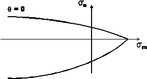
Fig. 2: The dependence of $Y$ on $\sigma_m$ expresses sensitivity to hydrostatic tension and corresponds to the meridian section of the yield surface.
The gradient of the boundary function $F$ in stress space has the form $$\frac{\partial F}{\partial\sigma_{ij}} = \frac{\partial\sigma_e}{\partial\sigma_{ij}}-\frac{\partial Y}{\partial\sigma_m}\frac{\partial\sigma_m}{\partial\sigma_{ij}}-\frac{\partial Y}{\partial\mu}\frac{\partial\mu}{\partial\sigma_{ij}}.\tag{4}\label{2-3}$$
In the special case of uniaxial stress, when $\sigma_{11}=\sigma$ and the other components of the stress tensor are zero, we get with respect to \eqref{1-10} \begin{align} \frac{\partial F}{\partial\sigma_{ij}} &= 0 \quad i\ne j,\\ \frac{\partial F}{\partial\sigma_{11}} &= \pm1-\frac{1}{3}\frac{\partial Y}{\partial\sigma_m},\tag{5}\label{2-4}\\ \frac{\partial F}{\partial\sigma_{22}} &= \frac{\partial F}{\partial\sigma_{33}} = \mp\frac{1}{2}-\frac{1}{3}\frac{\partial Y}{\partial\sigma_m}. \end{align}
Upper signs correspond to the case of uniaxial tension $\sigma>0$ and lower signs correspond to uniaxial compression $\sigma<0$.
Associative a non-associative creep rule
The direction of the plastic flow is specified by the direction tensor $R_{ij}$ $$\dot\varepsilon_{ij}^p = \lambda R_{ij},\quad \lambda>0.\tag{6}\label{3-1}$$
Most often used is the associative creep rule, when $$R_{ij} = \frac{\partial F}{\partial\sigma_{ij}}.\tag{7}\label{3-2}$$
According to \eqref{2-3} and by reducing \eqref{1-8}, the proportional change in volume corresponds to $$\dot\varepsilon_{kk}^p = \lambda\frac{\partial F}{\partial\sigma_{kk}} = -\lambda\frac{\partial Y}{\partial\sigma_m}.$$
For pressure-dependent yield criteria, $Y$ is decreasing with respect to $\sigma_m$, see Fig. 2. The derivative of $\partial Y/\partial\sigma_m$ is therefore negative and the associative creep rule implies a positive volume change. However, this prediction does not correspond to reality, and therefore the non-associative creep rule is sometimes used, most often in the form $$R_{ij} = \frac{3}{2}\frac{s_{ij}}{\sigma_e}+\Phi\delta_{ij}.\tag{8}\label{3-4}$$
The proportional change in volume is then $$\dot\varepsilon_{kk}^p = 3\lambda\Phi$$ and the quantity $\Phi$, which is called the dilation factor, can be set experimentally. If $\Phi=0$, \eqref{3-4} represents the Prandtl-Reuss equations with zero volume change.
Effective strain
We define the effective strain rate as $$\dot\varepsilon_p = \sqrt{\gamma\dot\varepsilon_{ij}^p\dot\varepsilon_{ij}^p},$$ where $\gamma$ is the definitoric parameter. According to \eqref{3-1} $$\dot\varepsilon_p = \lambda\sqrt{\gamma R_{ij}R_{ij}}$$ and the creep equation has the form $$\dot\varepsilon_p = \frac{\dot\varepsilon_p}{\sqrt\gamma}\rho_{ij},\quad \rho_{ij} = \frac{R_{ij}}{\sqrt{R_{kl }R_{kl}}}.\tag{9}\label{4-3}$$
We choose the parameter $\gamma$ so that with uniaxial tension $\sigma_{11}=\sigma$ holds $\dot\varepsilon_p=|\dot\varepsilon_{11}^p|$, or $$\gamma = \rho_{11}^2.\tag{10}\label{4-4}$$
For the associative creep rule, according to \eqref{2-4} we get $$\gamma = \frac{\left(\pm1-\frac{1}{3}\frac{\partial Y}{\partial\sigma_m}\right)^2}{\frac{3}{2} +\frac{1}{3}\left(\frac{\partial Y}{\partial\sigma_m}\right)^2}\tag{11}\label{4-5}$$ and for the non-associative rule \eqref{3-4} $$\gamma = \frac{(\pm1+\Phi)^2}{\frac{3}{2}+3\Phi^2}.\tag{12}\label{4-6}$$
The upper sign applies to the tensile calibration of the model (i.e., it applies to the case $\sigma_{11}>0$), while the lower sign corresponds to the compressive calibration (when $\sigma_{11}<0$). Compressive calibration was selected in the PMD system and lower signs apply in formulas \eqref{4-5}, \eqref{4-6}. In the special case of $\partial Y/\partial\sigma_m=0$ or $\Phi=0$, it is always $\gamma=2/3$.
For non-associative rule, regardless of the state of tension, $$R_{kl}R_{kl} = \frac{3}{2}+3\Phi^2,$$ so by substituting $\gamma$ (during pressure calibration) and $R_{kl}R_{kl}$ into \eqref{4-3} $$\dot\varepsilon_{ij}^p = \frac{\dot\varepsilon_p}{|1-\Phi|}R_{ij},$$ where $R_{ij}$ is given by the expression \eqref{3-4}. Using the $R_{ij}$ tensor, we get the relative volume change $$\dot\varepsilon_{kk}^p = \frac{3\Phi}{|1-\Phi|}\dot\varepsilon_p\tag{13}\label{4-9}$$ and the dilation factor $\Phi$ can be determined experimentally.
Combined hardening
For hardening materials, the yield criterion \eqref{2-1} is modified as follows: instead of the stress tensor $\sigma_{ij}$, the stress quantity $\tau_{ij}=\sigma_{ij}-h_{ij}$ is substituted where $h_{ij}$ is a tensor of kinematic parameters (backstress), and the dependence of the function $Y$ is expanded by the effective strain $\varepsilon_p$ $$F(\sigma_{ij}-h_{ij},\varepsilon_p,T) = \sigma_e-Y(\sigma_m,\mu,\varepsilon_p,T) = 0,\tag{14}\label{5-1}$$ while the invariants $\sigma_e$, $\sigma_m$, and $\mu$ are expressed for $\tau_{ij}$. It holds $$\frac{\partial F}{\partial\sigma_{ij}} = \frac{\partial F}{\partial\tau_{ij}} = -\frac{\partial F}{\partial h_{ij }}.\tag{15}\label{5-2}$$
The Prager model is used as the evolution equation for $h_{ij}$ $$h_{ij} = \kappa\frac{\partial F}{\partial\sigma_{ij}}.\tag{16}\label{5-3}$$
The function $Y$ can be decomposed into isotropic and kinematic components $$Y(\sigma_m,\mu,\varepsilon_p,T) = \sigma_Y(\sigma_m,\mu,\varepsilon_p,T)-Q_Y(\varepsilon_p),\tag{17}\label{5-4}$$ so by choosing $Q_Y(\varepsilon_p)$ we obtain different hardening models. Let’s denote $T_o$ the initial temperature corresponding to the state $\sigma_{ij}\equiv0$ and we have:
- Isotropic hardening $$Q_Y^\text{iso}(\varepsilon_p)\equiv0$$
- Kinematic hardening $$Q_Y^\text{kin}(\varepsilon_p)\equiv\sigma_Y(0,0,\varepsilon_p,T_o)-\sigma_Y(0,0,0,T_o)$$
- Kinematic-isotropic cyclic hardening $$Q_Y^\text{hrd}(\varepsilon_p)<Q_Y^\text{kin}(\varepsilon_p)$$
- Kinematic-isotropic cyclic softening $$Q_Y^\text{sft}(\varepsilon_p)>Q_Y^\text{kin}(\varepsilon_p)$$
During plastic flow, the consistency condition must be met $$\dot F = \frac{\partial F}{\partial\sigma_{ij}}\dot\sigma_{ij}+\frac{\partial F}{\partial h_{kl}}\dot h_{kl }+\frac{\partial F}{\partial\varepsilon_p}\dot\varepsilon_p+\frac{\partial F}{\partial T}\dot T = 0.\tag{18}\label{5-5}$$
We use the decomposition \eqref{5-4} and denote $$H' = \frac{\partial\sigma_Y}{\partial\varepsilon_p},\quad Q' = \frac{dQ_Y}{d\varepsilon_p}.$$
Substituting into \eqref{5-5} and using \eqref{5-2} we get $$\frac{\partial F}{\partial\sigma_{ij}}\dot\sigma_{ij}-\frac{\partial F}{\partial\sigma_{kl}}\dot h_{kl}-H '\dot\varepsilon_p+Q'\dot\varepsilon_p-\frac{\partial\sigma_Y}{\partial T}\dot T = 0.\tag{19}\label{5-7}$$
We further assume that the increment of the kinematic parameters depends exclusively on $Q'$, whence $$\frac{\partial F}{\partial\sigma_{kl}}\dot h_{kl} = Q'\dot\varepsilon_p$$ and the $\kappa$ multiplier in the Prager’s model \eqref{5-3} can be calculated as $$\kappa = \frac{Q'\dot\varepsilon_p}{g^2},\quad g^2 = \frac{\partial F}{\partial\sigma_{kl}}\frac{\partial F} {\partial\sigma_{kl}}.\tag{20}\label{5-9}$$
The consistency equation \eqref{5-7} simplifies to $$\frac{\partial F}{\partial\sigma_{ij}}\dot\sigma_{ij}-\frac{\partial\sigma_Y}{\partial T}\dot T = H'\dot\varepsilon_p. \tag{21}\label{5-10}$$
Generalized plasticity model
The yield criterion has the form \eqref{5-1} $$F(\sigma_{ij}-h_{ij},\varepsilon_p,T) = \sigma_e-Y(\sigma_m,\mu,\varepsilon_p,T) = 0.$$
We decompose the function $Y$ as v \eqref{5-4} $$Y(\sigma_m,\mu,\varepsilon_p,T) = \sigma_Y(\sigma_m,\mu,\varepsilon_p,T)-Q_Y(\varepsilon_p).$$
Prager’s kinematic hardening \eqref{5-3} and \eqref{5-9} gives $$\dot h_{ij} = Q'\frac{\dot\varepsilon_p}{g^2}\frac{\partial F}{\partial\sigma_{ij}}.$$
We write the creep rule in the general form \eqref{4-3} $$\dot\varepsilon_{ij}^p = \frac{\dot\varepsilon_p}{\sqrt\gamma}\rho_{ij},$$ where the unit direction tensor $\rho_{ij}$ follows from \eqref{3-2} or \eqref{3-4}.
It remains to determine $\dot\varepsilon_p,$ because then from Hooke’s law $$\dot\sigma_{ij} = D_{ijkl}(\dot\varepsilon_{kl}-\dot\varepsilon_{kl}^o-\dot\varepsilon_{kl}^p)\tag{22}\label {6-5}$$ the stress rate is obtained. The deformation $\dot\varepsilon_{kl}^o$ consists of a creep component and a thermal expansion with an expansion coefficient $\alpha$ $$\dot\varepsilon_{kl}^o = \dot\varepsilon_{kl}^c+\alpha\dot T\delta_{kl}$$ and is known in advance. By substituting \eqref{6-5} into the consistency equation \eqref{5-10} and solving with respect to $\dot\varepsilon_p$, we get $$\dot\varepsilon_p = \frac{\frac{\partial F}{\partial\sigma_{ij}}D_{ijkl}(\dot\varepsilon_{kl}-\dot\varepsilon_{kl}^o)- \frac{\partial\sigma_Y}{\partial T}\dot T}{H'+\frac{\partial F}{\partial\sigma_{mn}}D_{mnpq}\frac{\rho_{pq}} {\sqrt\gamma}}.$$
Isotropic creep model
For isotropic creep, we choose the unit direction tensor $\rho_{ij}$ fixed $$\dot\varepsilon_{ij}^c = \lambda\rho_{ij},\quad \rho_{ij} = \sqrt{\frac{3}{2}}\frac{s_{ij}}{\ sigma_e}.\tag{23}\label{7-1}$$
For uniaxial tension $\sigma_{11}=\sigma$, $\rho_{11}^2=2/3$, and according to \eqref{4-4} it holds for the parameter $\gamma=2/3=\text{ const.}$ The effective creep strain is therefore defined as $$\dot\varepsilon_c = \sqrt{\frac{2}{3}\dot\varepsilon_{ij}^c\dot\varepsilon_{ij}^c}$$ and under uniaxial tension it is $\dot\varepsilon_c=|\dot\varepsilon_{11}^c|.$ Substituting into \eqref{7-1} we have $$\dot\varepsilon_{ij}^c = \frac{3}{2}\frac{\dot\varepsilon_c}{\sigma_e}s_{ij}.$$
The creep strain rate $\dot\varepsilon_{ij}^c$ is now explicitly determined by the material state, since the dependence $$\dot\varepsilon_c = \dot\varepsilon_c(\sigma_e,\varepsilon_c,T)\tag{24}\label{7-4}$$ is subtracted from uniaxial creep curves. From the structure of the function \eqref{7-4}, it follows that the transition from one curve to another takes place at a constant effective strain $\varepsilon_c$, or according to the strain hardening hypothesis.
In PMD, the elastoplastic model and the creep model are combined according to the following rules:
- Inelastic deformation components are added, i.e., $$\varepsilon_{ij} = \varepsilon_{ij}^e+\alpha T\delta_{ij}+\varepsilon_{ij}^I,\quad \varepsilon_{ij}^I = \varepsilon_{ij}^p+\varepsilon_{ij}^c,$$ where $\varepsilon_{ij}^e$ is the elastic strain that can be calculated from the stress at any time using Hooke’s law, and $\varepsilon_{ij}^I$ is the permanent strain.
- The effective strains $\varepsilon_p$ and $\varepsilon_c$ are independent of each other.
Input quantities
The material quantities are defined in the file name.i2, while the quantities $\sigma_Y,Q_Y,{\dot\varepsilon}_c,\Phi$ are written on the 5th–8th position of the set:
MP set number T 1 V $E$ $\alpha$ $\nu$ $\rho$ $\sigma_Y$ $Q_Y$ ${\dot\varepsilon}_c$ $\Phi$
When defining material quantities, all functional dependencies can be used.
If some positions within the MP set are not used (see below), they must be formally written as 0.
The plasticity model is distinguished by the parameter $\mathtt{KMOD}$ in the file name.iP.
The creep calculation is activated by the parameter $\mathtt{KCRP}=1$ in the file name.iP regardless of the value of $\mathtt{KMOD}.$ For $\mathtt{KCRP}=1$ it is always necessary to enter dependence $\dot\varepsilon_c=\dot\varepsilon_c(\sigma_e,\varepsilon_c,T).$ If the creep deformation rate does not depend on $\varepsilon_c$, creep occurs in the area of secondary creep.
Elasticity ($\mathtt{KMOD}=0$)
Plastic constitutive relations are turned off, which can be used, for example, to calculate a separate creep problem.
Von Mises model — J₂ theory ($\mathtt{KMOD}=1$)
The function $\sigma_Y(\varepsilon_p,T),$ is specified, which can be calibrated on a uniaxial tensile test, when $\sigma_{11}=\sigma_Y(\varepsilon_{11}^p,T).$ If $\sigma_Y$ is only a function of the temperature $T$ or is constant, the material is considered ideally plastic. Next, the kinematic strengthening component $Q_Y(\varepsilon_p)$ is specified.
Generalized associative model ($\mathtt{KMOD}=2$)
The same as in the case $\mathtt{KMOD}=1$ is specified, but the function $\sigma_Y$ is extended by two stress invariants $\sigma_m$ and $\mu$. Dependence $\sigma_Y(\sigma_m,\ mu,\varepsilon_p,T)$ thus allows specifying any yield criterion. The function $\sigma_Y$ is calibrated on the case of uniaxial compression, for which $\sigma_{11}=\sigma_Y(\sigma_{11}/3,-1,\varepsilon_{11}^p,T).$
Generalized non-associative model ($\mathtt{KMOD}=3$)
The same as in the case $\mathtt{KMOD}=2$ is specified. In addition, it is necessary to specify the dilatation factor (volume expansion of plastic deformations) $\Phi$, which is calibrated using the equation \eqref{4-9}.


